Diagnostic visualization for causal estimands
CP plots and local CP plots in R.
CPplot draws estimated treatment effects against estimated propensity scores and returns the diagnostic linear fits used to read bracketing relationships and plug-in ATT, ATO, and ATC estimates.
Installation
install.packages("remotes")
remotes::install_github("e9tian/CPplot")
library(CPplot)Observational CP plot
If y is the outcome, z is the binary
treatment, and x is a covariate, a CP plot can be
drawn with cp_plot(y ~ z + x, data = df). The example
below uses three covariates in the same way.
Example
set.seed(1)
n <- 900
df <- data.frame(x1 = rnorm(n), x2 = rnorm(n))
p <- plogis(-0.30 + 1.05 * df$x1 - 0.45 * df$x2)
df$x3 <- p^2
df$z <- rbinom(n, 1, p)
tau <- -0.20 + 1.20 * p + 5.00 * df$x3 + 0.70 * df$x2
df$y <- 1 + 0.5 * df$x1 + 0.4 * df$x2 +
df$z * tau + rnorm(n, sd = 0.5)
fit <- cp_plot(y ~ z + x1 + x2 + x3, data = df)
fit$plot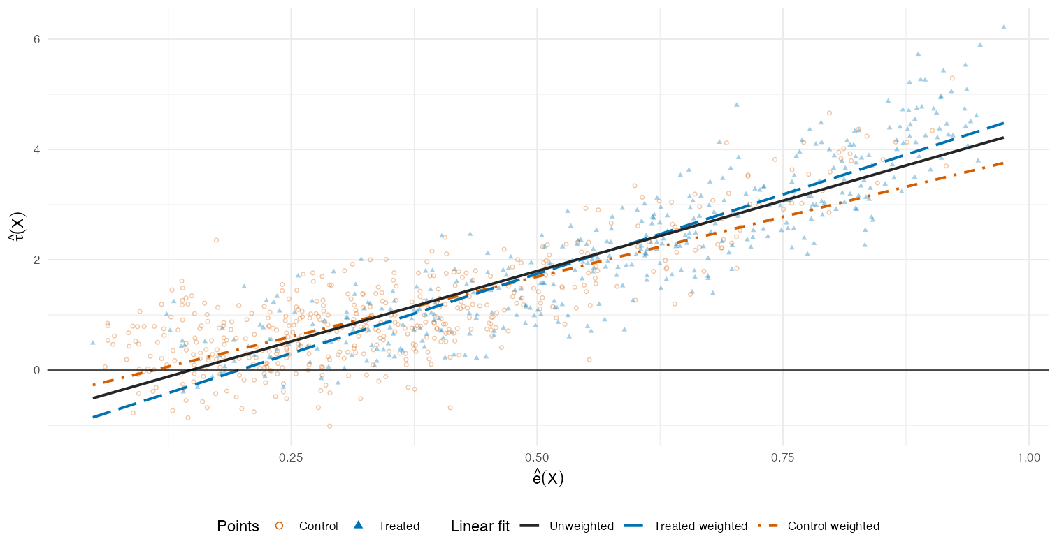
Numerical diagnostics
Use fit$slopes to report the fitted-line slopes and
fit$intersections to report the three pairwise
intersections and their plug-in ATT, ATO, and ATC estimates. Use
fit$bracketing to report the corresponding
bracketing implications. fit$bracketing_summary
gives a compact text summary of the ATO bracketing diagnostic.
fit$slopes
fit$intersections
fit$bracketing
fit$bracketing_summary# fit$slopes
fit n slope std_error p_value
1 Unweighted 900 5.101455 0.09159536 1.501789e-293
2 Treated weighted 900 5.760079 0.09442888 1.304333e-321
3 Control weighted 900 4.346009 0.10703058 1.776072e-205
# fit$intersections
estimand line_1 line_2 e_hat effect_hat
1 ATT Unweighted Treated weighted 0.5764895 2.186164
2 ATO Treated weighted Control weighted 0.4629750 1.532311
3 ATC Control weighted Unweighted 0.3640090 1.102205
# fit$bracketing
fit slope slope_sign implication
1 Unweighted 5.101455 positive ATT >= ATE >= ATC
2 Treated weighted 5.760079 positive ATT >= ATO
3 Control weighted 4.346009 positive ATO >= ATC
# fit$bracketing_summary
[1] "The tilted slopes support ATC <= ATO <= ATT."Local CP plot for IV studies
If y is the outcome, d is the treatment,
z is the binary IV, and x is a covariate,
a local CP plot can be drawn with
local_cp_plot(y ~ d + x | z + x, data = df). The
example below uses three covariates in the same way. In formula
mode, CPplot estimates the IV propensity score and both conditional
contrasts, then forms the plug-in inputs
pi_c_hat = delta_d and
tau_c_hat = delta_y / delta_d. By default,
points with z = 0 are labeled
Unencouraged, and points with z = 1 are
labeled Encouraged.
Example
set.seed(2)
n <- 900
df <- data.frame(x1 = rnorm(n), x2 = rnorm(n))
p <- plogis(-0.25 + 0.95 * df$x1 + 0.35 * df$x2)
df$x3 <- p^2
df$z <- rbinom(n, 1, p)
df$d <- rbinom(n, 1, plogis(-0.8 + 1.2 * df$z + 0.4 * df$x1 - 0.2 * df$x2))
tau <- -0.20 + 1.20 * p + 5.00 * df$x3 + 0.70 * df$x2
df$y <- 1 + 0.4 * df$x1 - 0.2 * df$x2 + tau * df$d + rnorm(n, sd = 0.5)
fit <- local_cp_plot(y ~ d + x1 + x2 + x3 | z + x1 + x2 + x3, data = df)
fit$plot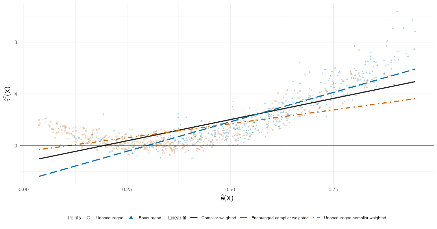
pi_c_hat, pi_c_hat * e_hat, and
pi_c_hat * (1 - e_hat).
Numerical diagnostics
Use fit$slopes to report the fitted-line slopes and
fit$intersections to report the pairwise line
intersections and their plug-in local ATT, ATO, and ATC estimates.
Use fit$bracketing to report the corresponding local
bracketing implications. fit$bracketing_summary
gives a compact text summary of the local ATO bracketing
diagnostic.
fit$slopes
fit$intersections
fit$bracketing
fit$bracketing_summary# fit$slopes
fit n slope std_error p_value
1 Complier weighted 900 6.541203 0.1677583 2.216206e-195
2 Encouraged-complier weighted 900 9.086877 0.1688588 3.131736e-283
3 Unencouraged-complier weighted 900 4.304402 0.1737031 1.034667e-103
# fit$intersections
estimand line_1 line_2
1 tau_ATT^c Complier weighted Encouraged-complier weighted
2 tau_ATO^c Encouraged-complier weighted Unencouraged-complier weighted
3 tau_ATC^c Unencouraged-complier weighted Complier weighted
e_hat effect_hat
1 0.5677469 2.462528
2 0.4683526 1.559344
3 0.3552332 1.072433
# fit$bracketing
fit slope slope_sign
1 Complier weighted 6.541203 positive
2 Encouraged-complier weighted 9.086877 positive
3 Unencouraged-complier weighted 4.304402 positive
implication
1 tau_ATT^c >= tau_ATE^c >= tau_ATC^c
2 tau_ATT^c >= tau_ATO^c
3 tau_ATO^c >= tau_ATC^c
# fit$bracketing_summary
[1] "The tilted slopes support tau_ATC^c <= tau_ATO^c <= tau_ATT^c."What the diagnostic lines tell you
Read the slope signs as diagnostics. A positive fitted slope gives the implication listed below; a negative fitted slope reverses the corresponding inequality.
| CP plot line | Weight used | Population analog | Positive slope implies |
|---|---|---|---|
| Unweighted linear fit | 1 |
cov{tau(X), e(X)} |
tau_ATT >= tau_ATE >= tau_ATC |
| Treated-weighted linear fit | e_hat_i |
cov{tau(X), e(X) | Z = 1} |
tau_ATT >= tau_ATO |
| Control-weighted linear fit | 1 - e_hat_i |
cov{tau(X), e(X) | Z = 0} |
tau_ATO >= tau_ATC |
| Local CP plot line | Weight used | Population analog | Positive slope implies |
|---|---|---|---|
| Complier-weighted linear fit | pi_c_hat_i |
cov{tau^c(X), e(X) | U = c} |
tau^c_ATT >= tau^c_ATE >= tau^c_ATC |
| Encouraged-complier weighted fit | pi_c_hat_i * e_hat_i |
cov{tau^c(X), e(X) | U = c, Z = 1} |
tau^c_ATT >= tau^c_ATO |
| Unencouraged-complier weighted fit | pi_c_hat_i * (1 - e_hat_i) |
cov{tau^c(X), e(X) | U = c, Z = 0} |
tau^c_ATO >= tau^c_ATC |
What the line intersections tell you
Theorem 3 of the associated paper shows that, when each corresponding pair of population projections is distinct, the vertical coordinate of each pairwise intersection is a weighted causal estimand. The horizontal coordinate is the corresponding propensity-score centroid.
fit$intersections reports
their analogs, and each vertical coordinate equals the corresponding
plug-in estimate.
| Pair of CP lines | Population intersection | Vertical coordinate |
|---|---|---|
| Unweighted and treated weighted | (e_bar_ATT, tau_ATT) |
ATT |
| Treated weighted and control weighted | (e_bar_ATO, tau_ATO) |
ATO |
| Control weighted and unweighted | (e_bar_ATC, tau_ATC) |
ATC |
Local CP plot
The same geometry holds under the complier distribution. The complier-weighted and encouraged-complier weighted lines intersect at the local ATT; the encouraged-complier and unencouraged-complier weighted lines intersect at the local ATO; and the unencouraged-complier and complier-weighted lines intersect at the local ATC.
| Pair of local CP lines | Vertical coordinate |
|---|---|
| Complier weighted and encouraged-complier weighted | tau_ATT^c |
| Encouraged-complier and unencouraged-complier weighted | tau_ATO^c |
| Unencouraged-complier and complier weighted | tau_ATC^c |
Already have fitted nuisance functions?
Pass fitted columns directly. This is useful after causal forests, BART, SuperLearner, xgboost, or your own estimator.
cp_plot(
data = df,
e_hat = "e_hat",
tau_hat = "tau_hat",
treatment = "z"
)
local_cp_plot(
data = df,
e_hat = "e_hat",
tau_c_hat = "tau_c_hat",
pi_c_hat = "pi_c_hat",
iv = "z"
)See the API reference for every argument, helper functions, and bundled paper-demo data.
Citation
citation("CPplot")Tian, P., Yang, F., & Ding, P. (2026). Introducing the CP-plot for Causal Inference with Observational Studies. arXiv preprint arXiv:2606.11715.